의사결정 나무 패키지
R에서는 의사결정 나무를 구현하기 위해서 다양한 패키지들을 제공합니다. 대표적으로는 rpart, tree, party가 있습니다.
이 패키지들의 차이점은 바로 "가치지기의 방법" 입니다.
- rpart: CART(classification and regression trees)을 사용합니다.
- tree: binary recursive partitioning을 사용합니다.
* 위 두개의 패키지들은 엔토로피와 지니계수를 사용해서 가치지기를 수행할 변수를 정합니다. 연산이 빠르다는 장점이 존재하지만 과적합될 가능성이 큽니다. 그래서 Pruning 과정을 통해서 과적합을 개선해 나가야 합니다.
- party: Unbiased recursive partitioning based on permutation test를 사용합니다. P-test를 거치게 된 중요도를 기준으로 가지치기 할 변수를 결정하기 때문에 별도의 가지치기 작업이 필요없습니다.
의사결정 나무 실습
1. 데이터 준비
credit<-read.csv("C:\\Users\\User\\Desktop\\머신러닝\\credit.csv")
head(credit)
 checking_balance months_loan_duration credit_history              purpose amount savings_balance
1           < 0 DM                    6       critical furniture/appliances   1169         unknown
2       1 - 200 DM                   48           good furniture/appliances   5951        < 100 DM
3          unknown                   12       critical            education   2096        < 100 DM
4           < 0 DM                   42           good furniture/appliances   7882        < 100 DM
5           < 0 DM                   24           poor                  car   4870        < 100 DM
6          unknown                   36           good            education   9055         unknown
  employment_duration percent_of_income years_at_residence age other_credit housing
1           > 7 years                 4                  4  67         none     own
2         1 - 4 years                 2                  2  22         none     own
3         4 - 7 years                 2                  3  49         none     own
4         4 - 7 years                 2                  4  45         none   other
5         1 - 4 years                 3                  4  53         none   other
6         1 - 4 years                 2                  4  35         none   other
  existing_loans_count       job dependents phone default
1                    2   skilled          1   yes      no
2                    1   skilled          1    no     yes
3                    1 unskilled          2    no      no
4                    1   skilled          2    no      no
5                    2   skilled          2    no     yes
6                    1 unskilled          2   yes      no
str(credit)
summary(credit)'data.frame': 1000 obs. of 17 variables:
$ checking_balance : Factor w/ 4 levels "< 0 DM","> 200 DM",..: 1 3 4 1 1 4 4 3 4 3 ...
$ months_loan_duration: int 6 48 12 42 24 36 24 36 12 30 ...
$ credit_history : Factor w/ 5 levels "critical","good",..: 1 2 1 2 4 2 2 2 2 1 ...
$ purpose : Factor w/ 6 levels "business","car",..: 5 5 4 5 2 4 5 2 5 2 ...
$ amount : int 1169 5951 2096 7882 4870 9055 2835 6948 3059 5234 ...
$ savings_balance : Factor w/ 5 levels "< 100 DM","> 1000 DM",..: 5 1 1 1 1 5 4 1 2 1 ...
$ employment_duration : Factor w/ 5 levels "< 1 year","> 7 years",..: 2 3 4 4 3 3 2 3 4 5 ...
$ percent_of_income : int 4 2 2 2 3 2 3 2 2 4 ...
$ years_at_residence : int 4 2 3 4 4 4 4 2 4 2 ...
$ age : int 67 22 49 45 53 35 53 35 61 28 ...
$ other_credit : Factor w/ 3 levels "bank","none",..: 2 2 2 2 2 2 2 2 2 2 ...
$ housing : Factor w/ 3 levels "other","own",..: 2 2 2 1 1 1 2 3 2 2 ...
$ existing_loans_count: int 2 1 1 1 2 1 1 1 1 2 ...
$ job : Factor w/ 4 levels "management","skilled",..: 2 2 4 2 2 4 2 1 4 1 ...
$ dependents : int 1 1 2 2 2 2 1 1 1 1 ...
$ phone : Factor w/ 2 levels "no","yes": 2 1 1 1 1 2 1 2 1 1 ...
$ default : Factor w/ 2 levels "no","yes": 1 2 1 1 2 1 1 1 1 2 ... checking_balance months_loan_duration credit_history purpose amount
< 0 DM :274 Min. : 4.0 critical :293 business : 97 Min. : 250
> 200 DM : 63 1st Qu.:12.0 good :530 car :337 1st Qu.: 1366
1 - 200 DM:269 Median :18.0 perfect : 40 car0 : 12 Median : 2320
unknown :394 Mean :20.9 poor : 88 education : 59 Mean : 3271
3rd Qu.:24.0 very good: 49 furniture/appliances:473 3rd Qu.: 3972
Max. :72.0 renovations : 22 Max. :18424
savings_balance employment_duration percent_of_income years_at_residence age
< 100 DM :603 < 1 year :172 Min. :1.000 Min. :1.000 Min. :19.00
> 1000 DM : 48 > 7 years :253 1st Qu.:2.000 1st Qu.:2.000 1st Qu.:27.00
100 - 500 DM :103 1 - 4 years:339 Median :3.000 Median :3.000 Median :33.00
500 - 1000 DM: 63 4 - 7 years:174 Mean :2.973 Mean :2.845 Mean :35.55
unknown :183 unemployed : 62 3rd Qu.:4.000 3rd Qu.:4.000 3rd Qu.:42.00
Max. :4.000 Max. :4.000 Max. :75.00
other_credit housing existing_loans_count job dependents phone default
bank :139 other:108 Min. :1.000 management:148 Min. :1.000 no :596 no :700
none :814 own :713 1st Qu.:1.000 skilled :630 1st Qu.:1.000 yes:404 yes:300
store: 47 rent :179 Median :1.000 unemployed: 22 Median :1.000
Mean :1.407 unskilled :200 Mean :1.155
3rd Qu.:2.000 3rd Qu.:1.000
Max. :4.000 Max. :2.000
> table(credit$default) no yes
700 300 default는 채무불이행을 했는지에 대한 여부를 나타냅니다. 즉 우리가 예측해야 될 값을 의미합니다. table 함수를 써서 확인해봤을때 전체의 30%는 채무 불이행을 한 것을 확인하였습니다.
# 시드값을 설정하면서 동인한 난수열을 따르게 설정한다.
set.seed(1234)
train_sample<-sample(1000,700)
str(train_sample)
학습데이터를 80% 테스트 데이터를 20%로 설정하였습니다.
train<-credit[train_sample,]
test<-credit[-train_sample,]
prop.table(table(train$default))
prop.table(table(test$default))
no yes
0.7014286 0.2985714 no yes
0.6966667 0.3033333 학습 데이터와 테스트 데이터를 완성 후 그 비율들을 비교해봤을때 비슷하게 할당이 된 것을 확인하였습니다.
2-1 모델 학습및 평가(rpart 패키지)
# rpart 패키지 사용
library(rpart)
tree_rp<- rpart(default~., data=train, method='class')
summary(tree_rp)
Call:
rpart(formula = default ~ ., data = train, method = "class")
n= 700
CP nsplit rel error xerror xstd
1 0.08612440 0 1.0000000 1.0000000 0.05793201
2 0.03827751 3 0.7416268 0.7416268 0.05256163
3 0.02551834 4 0.7033493 0.7272727 0.05219354
4 0.01674641 7 0.6267943 0.7272727 0.05219354
5 0.01435407 9 0.5933014 0.7320574 0.05231715
6 0.01196172 13 0.5358852 0.7607656 0.05303980
7 0.01116427 15 0.5119617 0.7559809 0.05292159
8 0.01000000 18 0.4784689 0.7703349 0.05327360
다음은 생성된 나무를 시각화를 해보도록 하겠습니다. rpart에서는 rpart.plot 패키지를 사용해서 시각화를 진행할 수 있습니다.
library(rpart.plot)
install.packages("rpart.plot")
library(rpart.plot)
rpart.plot(tree_rp)
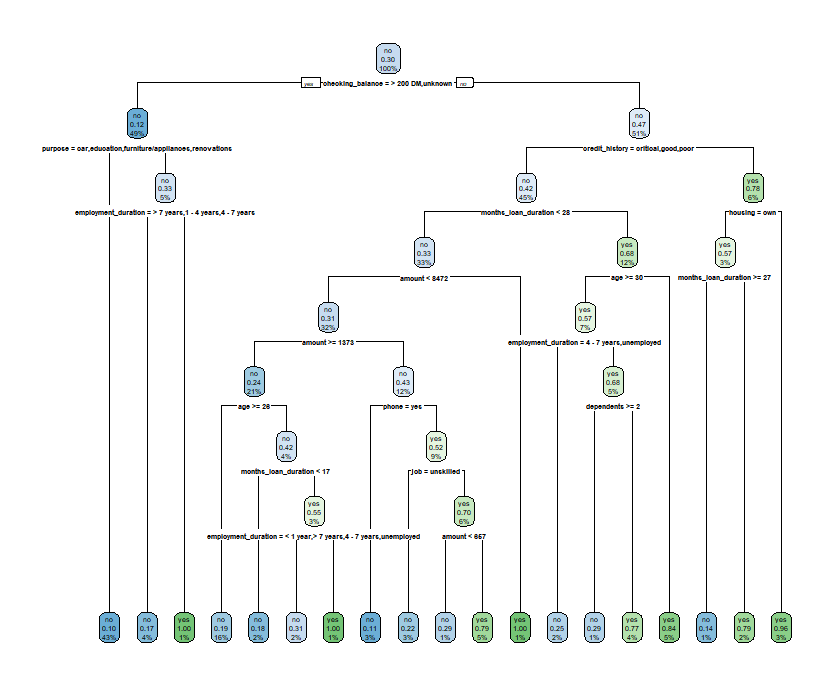
위에서 말했듯이 rpart 패키지는 과적합의 위험성이 크다고 하였습니다. 이 부분을 해결하기 위해서 가치지기를 수행 하도록 하겠습니다. 이때 사용되는 함수는 print.cp 함수입니다.
printcp(tree_rp)
Classification tree:
rpart(formula = default ~ ., data = train, method = "class")

Variables actually used in tree construction:
 [1] age                  amount               checking_balance     credit_history
 [5] dependents           employment_duration  housing              job
 [9] months_loan_duration phone                purpose

Root node error: 209/700 = 0.29857

n= 700

        CP nsplit rel error  xerror     xstd
1 0.086124      0   1.00000 1.00000 0.057932
2 0.038278      3   0.74163 0.74163 0.052562
3 0.025518      4   0.70335 0.72727 0.052194
4 0.016746      7   0.62679 0.72727 0.052194
5 0.014354      9   0.59330 0.73206 0.052317
6 0.011962     13   0.53589 0.76077 0.053040
7 0.011164     15   0.51196 0.75598 0.052922
8 0.010000     18   0.47847 0.77033 0.053274
plotcp(tree_rp)
xerror 값이 가장 낮은 split값을 선택하면 되는데요. 결과값과 그래프를 보면 7에서의 split에서 가장 낮은 값을 나타냅니다. split 7에서 cp값은 0.016746 이므로 대략 cp값을 0.02로 설정해 보겠습니다.
rpart_pr<-prune(tree_rp, cp=0.02)
rpartpred<-predict(rpart_pr, test, type='class')
confusionMatrix(rpartpred, test$default)
Confusion Matrix and Statistics
Reference
Prediction no yes
no 169 57
yes 40 34
Accuracy : 0.6767
95% CI : (0.6205, 0.7293)
No Information Rate : 0.6967
P-Value [Acc > NIR] : 0.7936
Kappa : 0.1924
Mcnemar's Test P-Value : 0.1043
Sensitivity : 0.8086
Specificity : 0.3736
Pos Pred Value : 0.7478
Neg Pred Value : 0.4595
Prevalence : 0.6967
Detection Rate : 0.5633
Detection Prevalence : 0.7533
Balanced Accuracy : 0.5911
'Positive' Class : no
Confusion Matrix를 통해 성능 평가를 해본 결과 정확도는 약 0.67정도로 나타났습니다.
2-2 모델 학습및 평가(tree 패키지)
사용되는 패키지명은 tree 입니다.
install.packages("tree")
library(tree)
tree_tr<-tree(default~. , data=train)
summary(tree_tr)
Classification tree:
tree(formula = default ~ ., data = train)
Variables actually used in tree construction:
[1] "checking_balance" "purpose" "employment_duration" "credit_history"
[5] "months_loan_duration" "amount" "housing"
Number of terminal nodes: 8
Residual mean deviance: 0.9198 = 636.5 / 692
Misclassification error rate: 0.2 = 140 / 700
다음은 트리를 시각화를 해보겠습니다.
plot(tree_tr)
text(tree_tr)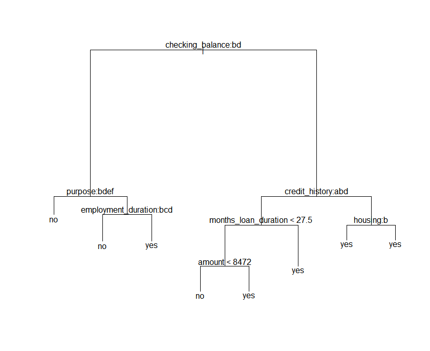
트리는 이러한 구조를 가지고 있습니다. tree 패키지도 rapart와 동일하게 가지치기 과정이 필요합니다. 이때 사용되는 함수는 cv.tree함수를 사용해서 split개수를 정하도록 하겠습니다.
cv.tree<-cv.tree(tree_tr, FUN=prune.misclass) 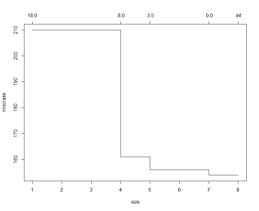
분산값이 가장 작은 7로 split수를 지정하도록 하겠습니다.
prune_tree<-prune.misclass(tree_tr, best=7)
plot(prune_tree)
text(prune_tree)
트리를 시각화 해보니 이전보다 간단해진것을 알 수 있습니다.
Confusion Matrix and Statistics

          Reference
Prediction  no yes
       no  180  66
       yes  29  25

               Accuracy : 0.6833
                 95% CI : (0.6274, 0.7356)
    No Information Rate : 0.6967
    P-Value [Acc > NIR] : 0.7158895

                  Kappa : 0.1536

 Mcnemar's Test P-Value : 0.0002212

            Sensitivity : 0.8612
            Specificity : 0.2747
         Pos Pred Value : 0.7317
         Neg Pred Value : 0.4630
             Prevalence : 0.6967
         Detection Rate : 0.6000
   Detection Prevalence : 0.8200
      Balanced Accuracy : 0.5680

       'Positive' Class : no
성능 평가를 해본 결과 정확도가 약 0.68로 rpart보다 약간 높은 예측률을 나타냈습니다.
2-3 모델 학습및 평가(party 패키지)
사용되는 패키지명은 party 입니다.
# party 패키지 사용
install.packages("party")
library(party)
tree_pt<-ctree(default~., train)
plot(tree_pt)
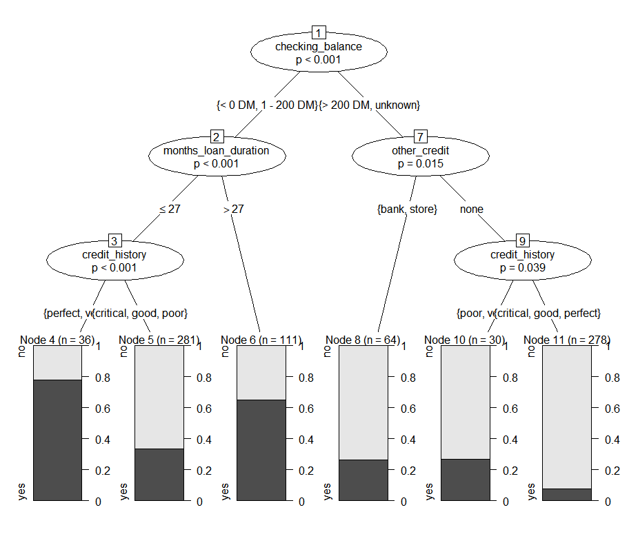
트리는 다음과 같이 생겼습니다. 앞의 예제들과는 약간 다른 시각화 모양이 나오는 것을 알 수 있습니다.
party패키지는 따로 가치치기 과정이 필요 없다고 앞에서 언급하였습니다. 따라서 바로 테스트를 하고 성능 평가를 진행 하도록 하겠습니다.
partypred<-predict(tree_pt, test)
confusionMatrix(partypred, test$default)
Confusion Matrix and Statistics

          Reference
Prediction  no yes
       no  181  66
       yes  28  25

               Accuracy : 0.6867
                 95% CI : (0.6309, 0.7387)
    No Information Rate : 0.6967
    P-Value [Acc > NIR] : 0.6722447

                  Kappa : 0.1596

 Mcnemar's Test P-Value : 0.0001355

            Sensitivity : 0.8660
            Specificity : 0.2747
         Pos Pred Value : 0.7328
         Neg Pred Value : 0.4717
             Prevalence : 0.6967
         Detection Rate : 0.6033
   Detection Prevalence : 0.8233
      Balanced Accuracy : 0.5704

       'Positive' Class : no
성능 평가 결과 앞의 두 패키지들보다 정확도가 약간 높게 나왔습니다. 최종적으로는 party>tree>rpart순으로 성능이 좋게 나왔습니다.
하지만 모든 데이터에서 그러한 결과가 나오는 것은 아닙니다. 따라서 의사결정나무는 패키지 종류가 다양하기 때문에 데이터의 구조와 특징에 맞게 그 결과를 비교해서 가장 좋은 예측을 나타내는 패키지를 선택하는 것이 중요합니다.
'Machine Learning' 카테고리의 다른 글
| 회귀란? (0) | 2020.05.26 |
|---|---|
| ML 평가 지표 (0) | 2020.05.09 |
| K-NN 알고리즘 (0) | 2020.05.05 |
| 분류 실습(신용카드 사기 데이터) (0) | 2020.05.03 |
| LightGBM (3) | 2020.04.28 |


